Intro
In the previous blog, I did forward kinematics, and this week, I worked on
- An easy version of inverse kinematics
- Code cleanup
- Setting up a system to control the Arduino via Matlab instead of python
This inverse kinematics implementation took 2 hours. It’s not that good, but it was VERY easy to implement.
The goal with inverse kinematics is to take the desired location/orientation of the end effector as input and find the joint angles + displacements needed to get to this location. This is more complicated than forward kinematics due to the possibility of multiple solutions or no solutions. An example of multiple solutions would be an arm with extra degrees of freedom being able to get to the same orientation in multiple different ways. Some examples of no solutions would be a position that is far away from the arm and therefore out of reach, or a position that the arm can not get to without colliding with itself.
A common easy method is using the Jacobian, but I did not fully understand it at first, so I tried something else that actually works in a similar way. I understood gradient descent from neural networks and my Calculus 3 course, so I used that instead.
Gradient Descent
You have a set of inputs (angles) and a set of outputs (xyz position), which are a function of the inputs (forward kinematics). You want to get certain outputs (the target/desired position), but do not know what inputs you need to give to get this output.

So what you do is create a cost function. This cost function outputs a cost/error, and, when set up correctly, this cost goes down the closer you get to your outputs. For us, this cost function is the distance formula.

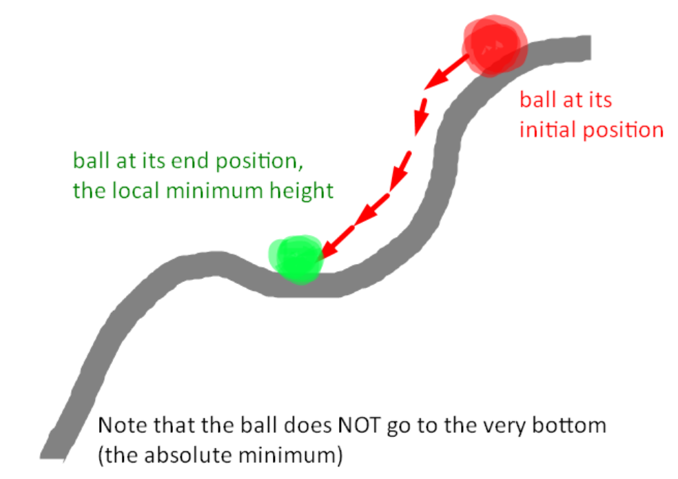
As you get closer to the target position, the cost (distance) goes down. You can now take the gradient of the cost function. The gradient points in the direction you need to move to get the highest rise in the cost function. Since we want to minimize our cost function, we move a tiny distance in the opposite direction. We are now slightly closer to the local minimum of our cost function, and assuming a correctly made cost function, our ideal output. How would code do this?
- Calculate the cost (distance) for the current inputs (angles).
- Try adding a tiny value (called the step size/learning rate) to one of the inputs and recalculate the cost. If the cost is lower, you were moving in the right direction. Regardless, store the change in cost for this input in a variable.
- Do for all inputs.
- Subtract from each input the step size multiplied by the change in cost for that input.
- Repeat cycle.
This will get you closer and closer to your target position with every iteration. You can kind of imagine this as dropping a ball on a hill. The ball will move down the hill towards the local minimum height. Of course, since we have many inputs rather than 1 input, we can not visualize our exact problem, since it will be many dimensional.

I might not have explained it too well, but in reality its quite simple. It only took me two hours to implement this, and the results are OK.

The Matlab code for the inverse kinematics is here
The Kinematics.invKPosition2 function is in this file
There are a few differences here. The main one is the cost function, which is the distance squared rather than the distance. This is to avoid the square root calculation. Since it still decreases the closer you get to the target, it still works as a cost function.
The other difference is the usage of the Kinematics.simulateTravel function to limit the rate of change. This is purely for us to get a realistic simulation. Without this, the angles would very rapidly change too quickly for us to see.
Next Time
I thought inverse kinematics would be much harder to get working, but now I realize that a simple implementation is not hard. What is actually hard is dealing with multiple or no solutions, limited ranges, local minimums, etc. So inverse kinematics requires a lot of messing around with different methods and tuning. I am limited by my math knowledge, but I want to try more things. Two ideas I have now are Jacobian and neural networks.
Using Jacobian is more direct than gradient descent.
Neural networks will be able to learn how to deal with specific arms. They have the ability to store information in their nodes via training. It is useful here for taking into account details that are unique to each arm, such as limited angle ranges (ex. 0–180) and collision between the arm and itself.
I can also improve on the gradient descent method.
I originally wanted to use the arm to learn inverse kinematics, and control it via python. However, after using Matlab, I found that it was very easy to simulate arms in Matlab. So I will probably forget about dealing with the arm until a long time later, or altogether. The calibration challenges would be easier on a better arm anyway (one with encoders), so I could just delay that until I have access to a better arm. I could also just use a simulated arm, randomly change the values, and use that instead of a real arm. This would be much faster for generating datasets as well.
I also found out that I can control the arduino much more easily in Matlab via the arduino library, without needing to code the arduino at all. This combined with my code already being in Matlab made me choose to stop using Python, although I may use it in the future for Tensorflow. If I continue working on the physical arm, it will be through Matlab.