Intro
The goal with this project is to learn to control a robot arm. I will be primarily focused on
- Forward Kinematics
- Inverse Kinematics
- Calibration
This blog will be on forward kinematics.
The Arm
I made a simple 3 axis arm in a few hours out of toy servos and popsicle sticks.
I realized later that I can only give the servos the angles I want them to move to, and am unable to sense the current angle without adding a sensor or modifying the servo. So while I can order the servo to try to move to a position, I will probably not be able to sense the arm’s location without some sort of vision + depth sensing, because any physical contact with the very weak toy arm will move it, and I can not sense that movement. This makes calibration much harder, so I will probably end up not using this arm for calibration experiments. I might also just replace the arm entirely with a better arm.
Forward Kinematics Explained
The goal with forward kinematics is to find the location/orientation of the end effector of an arm with joint angles + displacements as input. The goal with inverse kinematics is to take the desired location/orientation of the end effector as input and find the joint angles + displacements needed to get to this location.
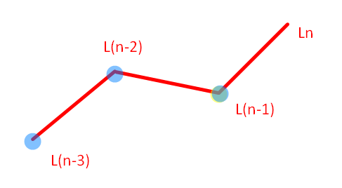
For forward kinematics, we have vectors in a position/orientation relative to the end effector, and we want the vectors in a position/orientation relative to the base of the robot. We need to get a transformation matrix that brings us from the end effector to the previous link, Ln to L(n-1).

Two prerequisites were important for me to understand. First we need to understand rotation matrices. Here is an example of a 2d rotation matrix that rotates a given vector counterclockwise by θ around the origin. Click the link in the caption to see more of them, such as 3D ones. Its mainly important to be able to recognize the form for when it appears in the matrices later.

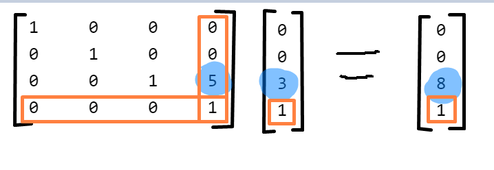
The second prerequisite is how to do addition (translation) via matrix multiplication. This is actually very simple, you just add an extra row and column. What is in the extra column is added on multiplication. Look at the blue highlighted numbers to understand. A 3x3 matrix and a 3x1 vector is extended to 4x4 matrix and a 4x1 vector. By using the extra columns, we can add via matrix multiplication.

Those are the requirements done. For the forward kinematics, I used Denavit Hartenberg (DH) convention since it seems like the most common convention. It uses 4 parameters to change frame, θ, r, α, and d. This video is much better at explaining it than any explanation with words or pictures. https://www.youtube.com/watch?v=rA9tm0gTln8
Varying θ or d allows us to rotate or translate. If we want to do multiple rotations or translations in a joint, we can use multiple joints in the same location with zero length links connecting them.
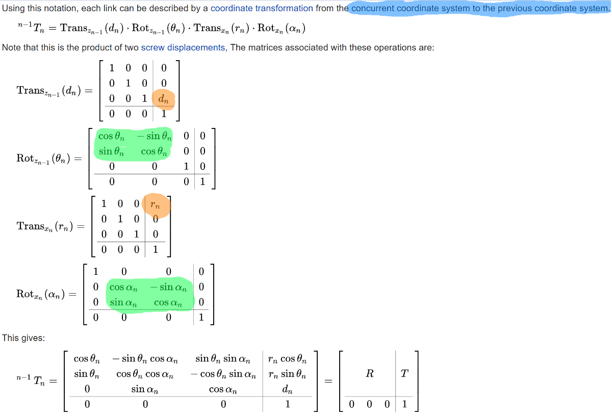
This is a screenshot from Wikipedia of the matrices for the transformation with some highlights.

With our prerequisite knowledge of how to do/recognize rotation and translation and what the DH parameters are, these formulas make sense, since we can easily see the rotation parts (sets of sine and cosine highlighted in green) and the translation parts (last column of the matrices highlighted in orange). The final combined matrix can be multiplied with a vector in the current frame to get the same vector in relation to the previous frame (the previous link), allowing us to move backwards from the end effector to the base of the arm.
Matlab
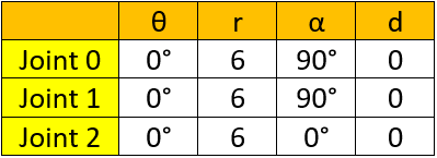
I made a 3 axis arm in Matlab (different from the real arm I made). Here are the parameters.

With these parameters and some Matlab code that took a surprisingly long time to get working, I got a simple simulation. All three joints have their θ increasing from 0 to 360:

The points needed to draw the lines were found with the forward kinematics as described before. In a function, I looped backwards through an array of link parameters, created the full transformation matrix for each one, and multiplied them together.
        % forward kinematics (get the transformation T)
        function [T] = fwk(P)
                T = eye(4);
                for i1=size(P,1):-1:1
                    theta = P(i1,1);
                    alpha = P(i1,2);
                    r = P(i1,3);
                    d = P(i1,4);
                    A = [
                        cosd(theta),-sind(theta)*cosd(alpha),sind(theta)*sind(alpha),r*cosd(theta);
                        sind(theta),cosd(theta)*cosd(alpha),-cosd(theta)*sind(alpha),r*sind(theta);
                        0,sind(alpha),cosd(alpha),d;
                        0,0,0,1
                        ];
                    % we need to transform link by link from end effector to the base
                    % So add it on
                    T = A*T;
                end
        end
Conclusion
That is all for this blog. Future blogs in this project will involve inverse kinematics and if possible calibration.
The Kinematics.fwk function is in this file.
Here is the code for the simulation.
Here are all the links I found useful for learning: